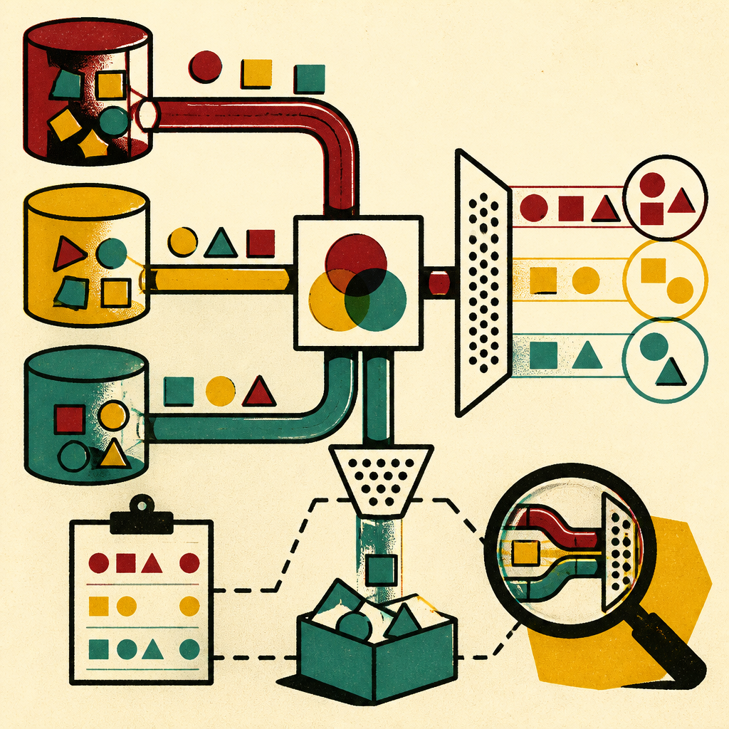
Data Pipeline: Sample-Construction Flow Diagram

Read the code that builds a project's analysis dataset and turn it into a diagram that shows exactly how the sample was constructed: which raw datasets went in, what key each merge joined on, how many rows matched versus fell out, why the unmatched rows did not match, and every filter that dropped observations — all the way from the initial raw counts down to the final estimation sample.

The output is the "sample-selection" or "data provenance" figure that reviewers at management and strategy journals increasingly ask for, and a companion table that makes every count reproducible.

When This Skill Is Invoked

The user wants to see, document, or verify how their analysis sample was built. Required input:

• Path to the pipeline code — a single script, or a directory of scripts, that reads raw data, merges it, filters it, and writes an analysis dataset (e.g., code/01_build_sample.R, code/clean/, do/merge.do).

Optional inputs:

• --language R|python|stata — which language the pipeline is written in. Infer from file extensions if not given.
• --format mermaid|tikz|dot — diagram output format. Default to mermaid for a first pass (fast to render and iterate), then offer tikz for a paper-ready figure. See Step 5.
• A hint about where the pipeline starts and ends (e.g., "starts from the raw Compustat pull, ends at analysis_panel.rds") if the entry and exit points are not obvious.

---

Step 1: Locate and Order the Pipeline

Find the code that constructs the sample and put it in execution order.

• Glob for build/clean/merge scripts and read them. Look for the files that read raw data and write an analysis dataset — not the estimation code.
• If there are multiple scripts, establish the order: a numbered prefix (01_, 02_), a master run/makefile/_targets.R, or source()/do/import calls between scripts.
• Identify the two anchors of the diagram: the raw source datasets (where rows first enter) and the final analysis sample (the dataset handed to estimation). Everything in between is what you are tracing.

State the ordered list of files back to the user before going further, so a wrong entry point gets caught early.

---

Step 2: Extract the Pipeline Structure

Read the code and build a step-by-step model of what happens to the rows. You are looking for four kinds of operation. For each, record the fields listed.

Source load — a raw dataset enters the pipeline.

• Dataset name, file path, and source (Compustat, hand-collected, survey wave, etc.)
• Unit of observation (firm-year, person, patent, transaction)
• The key variable(s) that identify a row

Merge / join — two inputs are combined on a key.

• The join key(s), spelled out exactly as they appear in the code
• Join type: 1:1, 1:many, many:1, or many:many. Flag every many:many explicitly — it is the most common source of silent row explosions.
• Which input is "left" (the spine you are keeping) and which is "right"
• What the code does with non-matching rows: inner join (drops both sides' non-matches), left join (keeps left, right-only lost), full join, etc. Translate the code's verb (merge, left_join, inner_join, m:1, pd.merge(how=...)) into match/no-match behavior. If some observations are unmatched and dropped from the sample, investigate whether this is a genuine non-match or error in the matching variables. Produce some examples of non-matched rows, and try to identify possible reasons for non-match. For example, the matching variable might have been coded differently across subsets, fuzzy matches might have not worked for a certain string format, the matching variable might be missing for a certain subset for some reason, or the data type might have been mismatched. If you find potential errors with the merge, move upstream of the code to identify any mistakes made in prior steps.

Filter / drop — rows are removed by a condition.

• The condition, in plain language and as it appears in code (filter(year >= 2000), drop if missing(roa), dropna(subset=...))
• The reason the rows are being dropped — infer it from the condition, variable names, and any nearby comment (out of window, missing key covariate, non-operating firm, duplicate, failed a validity check). This "why" is the point of the diagram; do not skip it.

Transform that changes N — a collapse, aggregate, reshape, or de-duplication that changes the row count without an explicit filter.

• What operation, at what grain, and whether it aggregates (fewer rows) or reshapes long/wide (row count changes meaning).

Watch for the subtle count-changers that are not written as filter: distinct() / duplicates drop, group_by |> summarise, collapse, a many:many merge, na.omit() on the whole frame, and drop_na() with no subset. These silently move the count and belong on the diagram.

---

Step 3: Get the Actual Observation Counts

A diagram with real numbers is worth ten with placeholders. Try, in this order, to attach a true row count to every node.

1. Read existing logs or output. If the pipeline already prints counts, a Stata .log, or an _merge tabulation, harvest those numbers first.
2. Run or instrument the code. If the raw data is available and the pipeline runs, execute it and capture N at each step. The clean way is to add lightweight count probes after each load, merge, and filter rather than eyeballing — insert nrow() / dim / count prints (R: dplyr::count() or nrow(); Python: len(df); Stata: count and tab _merge) at each boundary, run once, and collect the trace. Keep the probes in a scratch copy so you never modify the user's script in place unless they ask.
3. Capture the merge split, not just the total. For every merge, get three numbers, not one: matched, left-only (master unmatched), and right-only (using unmatched). In Stata this is tab _merge (codes 1/2/3). In R, compare pre-join nrow against an anti-join both directions. In pandas, merge with indicator=True and tabulate _merge. The unmatched counts are what the reader most wants to see.
4. If the code cannot be run, say so plainly, mark the counts as unknown, and still produce the structural diagram with the boxes and reasons in place. Do not invent numbers. A labeled "N = ?" is honest; a fabricated count is a landmine.

Whenever you get a matched/unmatched split, also try to characterize why the unmatched rows did not match — spot-check a handful of the failing keys (wrong identifier vintage, name vs. code mismatch, out-of-coverage period, trailing whitespace, a . vs. missing). One sentence of diagnosis per merge is the difference between a figure and a footnote.

---

Step 4: Reconcile the Arithmetic

Before drawing anything, make the counts add up. For every step: rows in − rows dropped (or − right-only, for an inner merge) = rows out. Walk the whole chain and confirm the final node equals the initial minus everything shown falling out the sides.

If it does not reconcile, there is a hidden count-changer you missed in Step 2 — usually a duplicate-dropping merge or an implicit na.omit. Find it and add it as its own node rather than fudging a number. Report any gap you cannot close; an unexplained delta is itself a finding worth surfacing to the user.

---

Step 5: Draw the Diagram

Build a top-to-bottom flow. The main spine is the shrinking analysis sample: each box carries a short label and its N. Side branches peel off to the right for every dropped or unmatched group, each labeled with its count and its reason. This is the CONSORT-diagram convention, adapted for observational data construction, and it is what readers already know how to read.

Conventions that keep it legible:

• Put the running sample count in every spine box (Firm-years, N = 48,213).
• Label each downward arrow with the operation (merge on gvkey-year, keep 2000–2019).
• Send drops sideways, never down, and label the branch with both the count and the reason (− 2,104: no match in Compustat (private firms)).
• On merge nodes, name the key and the join type. Show right-only rows as their own side branch when they are lost.
• End at a clearly marked terminal node: the final analysis sample and its N.

Emit the format the user asked for; default to Mermaid for the first pass.

• Mermaid (flowchart TD) — renders in the terminal preview and in GitHub/markdown, so it is the fastest to iterate on. Best for review and for the repo's README.
• TikZ — paper-ready, matches a LaTeX manuscript, fully styleable. Offer this once the structure is settled. Use a matrix of nodes with -> edges, or the smartdiagram/forest style if the user already uses one. Compile it to a standalone PDF to check it renders.
• Graphviz DOT — good middle ground when the user wants a PNG/PDF without LaTeX; render with dot -Tpdf.

Write the diagram source to figures/sample_construction.<ext> (create the directory if needed) so it lives with the project, and render it if the toolchain is available. Keep the diagram source small and readable — the user maintains it after you.

---

Step 6: Report

Summarize for the user:

• The path from initial raw counts to the final sample, in one or two sentences ("Started at 61,402 firm-years across three sources; the final panel is 41,880 after dropping private-firm non-matches, pre-2000 years, and firm-years missing ROA").
• Where the biggest losses happened, and whether any of them look like a threat to inference (e.g., a merge that drops 30% of rows non-randomly, a many:many join that inflated the count, a filter that silently removed a whole subgroup).
• Anything that did not reconcile, or any count that could not be obtained.
• The files written: diagram source, rendered figure, and provenance table.

Flag as a concern, not just a note, any of: a many:many merge, an unmatched share above ~10% that is not explained, a filter whose reason you could not determine, or a count gap you could not close. These are the sample-construction problems that sink papers in review.

---

Language-Specific Notes

R — Merges: dplyr::*_join, merge(), data.table X[Y] and merge(), fuzzyjoin. Get splits with anti_join() both directions or dplyr::*_join(..., keep = TRUE). Counts: nrow(), dplyr::count(), janitor::tabyl. Watch distinct(), summarise() after group_by(), na.omit(), tidyr::drop_na().

Python / pandas — Merges: pd.merge, df.join, df.merge(..., indicator=True) then value_counts() on _merge for the split. Counts: len(df), df.shape[0]. Watch drop_duplicates(), groupby().agg(), dropna(), and chained filters.

Stata — Merges: merge 1:1 / m:1 / 1:m / m:m — always read tab _merge (1 = master only, 2 = using only, 3 = matched). Counts: count, count if. Watch duplicates drop, collapse, keep if / drop if, reshape, and any merge, keep(match).

---

Quick Reference

Step	What it does	Key output
1 Locate	Order the build scripts, find entry/exit	Ordered file list
2 Structure	Extract loads, merges, filters, transforms	The pipeline model
3 Counts	Run/instrument to get true N and merge splits	Matched / left-only / right-only
4 Reconcile	Make the arithmetic close	No unexplained deltas
5 Diagram	Draw spine + side branches, initial → final	figures/sample_construction.*
6 Report	Summarize losses and flag threats	Concerns surfaced